
📌 Highlights
The paper measures whether temporal defects in generated visual continuations are linearly decodable from a fixed model of the fly visual system. The observer was trained for optic-flow estimation and receives MPI-Sintel luminance rendered on its 721-column retina; a logistic-regression two-sample test compares temporal statistics of its cell-type responses to real windows and generated continuations. This tests a response representation, rather than asking the observer itself to make a decision.
Across three generators and three temperatures, the trained observer’s AUC ranges from 0.85 to 0.99. For learned world models, the corresponding untrained network produces AUCs of 0.58–0.75, with paired trained-minus-untrained differences of 0.20–0.37. The study also reports similar separability on sequences the observer did not see during training. These findings describe this dataset, observer, and classifier setup.
The graded probes make the result more specific: swapping one adjacent pair of real frames gives AUC 0.73 for trained responses, versus 0.54 for the untrained network and 0.56 for pixel statistics. The authors interpret the evidence as temporal defects becoming available in trained responses. It does not show that a fly detects dreams, and the connectome’s specific contribution is not isolated.
- Main task: distinguish real MPI-Sintel windows from world-model continuations using temporal response statistics.
- Reported comparison: trained-observer AUC 0.85–0.99 across nine conditions; low-temperature MDN-RNN is hardest at full length.
- Key caveat: classifier separability is not biological perception or behavior.
🎯 Introduction
The paper frames a measurable version of the question of whether a fixed visual system can distinguish a generated continuation from reality. Its focus is the observer model: a connectome-constrained fly visual-system network trained on optic-flow estimation. The authors ask what this task training makes available in the network’s responses beyond the trained task, when the model sees continuations made by a separate world model.
The motivation is that generated continuations can resemble real context frame by frame yet depart in temporal structure, and the observer was not trained to detect those departures. Prior world-model work uses generated rollouts as an environment for control, where less faithful rollouts can sometimes help transfer. That purpose differs from the present evaluation question: whether a fixed observer’s responses make differences between generated and real sequences linearly decodable.
The paper operationalizes “can tell” as a classifier two-sample test on temporal statistics of cell-type responses, with the observer held fixed. It compares trained responses against the same network before training and against direct luminance statistics. This design tests whether the trained response space exposes differences in the selected stimuli; it does not establish that the connectome alone causes the effect or that an animal would report the difference.
🔬 Methodology
The observer is flyvis version 1.2.0, a hexagonal-lattice optic-lobe model whose connectivity follows the connectome. It contains 45,669 cells of 65 types and has 734 free parameters trained by the model’s authors for optic-flow estimation. The study uses all 50 released trained models without modification. Its untrained control restores no checkpoint and retains the connectome’s signs and synapse counts; five seeds differ in their cell-type bias draws.
Reality consists of MPI-Sintel luminance sequences rendered with the observer’s preprocessing to 721 columns. The paper forms 198 non-overlapping 19-frame windows. Each dream keeps five real context frames and generates 14 continuation frames in the same input space. The three generators are a persistence random walk, an MDN-RNN with an LSTM and mixture-density head, and an RSSM with deterministic and stochastic latent states. Each is tested at temperatures 0.25, 0.5, and 1.0.
For each cell type, the main analysis aggregates responses across cells and computes the mean, standard deviation, lag-1 autocorrelation, and mean absolute step-to-step change over generated frames. These four statistics across 65 types form a 260-dimensional feature vector. An ℓ2-regularised logistic regression separates real windows from one dream condition at a time; dream is positive and AUC 0.5 indicates indistinguishability. The generator and classifier folds keep sequences disjoint, and confidence intervals use sequence-cluster bootstrap. A luminance control applies the temporal statistics to 65 principal components fitted on real training frames.
The persistence baseline is specified by the source equation below. Its noise scale is set per fold so that at temperature 1 its expected frame change matches the training series. The authors additionally evaluate detection horizons using only the first k generated frames and construct graded probes that swap adjacent pairs or repeat real frames. Those probes isolate temporal-order perturbations from the particular generative model.
Persistence random walk
Meaning: Defines the no-learning continuation baseline: per-column Gaussian perturbations are scaled by temperature and calibrated noise scale, then clipped to the input range.
📊 Experiments
The empirical evaluation uses MPI-Sintel: 35 sequences, yielding 198 windows, including 17 sequences seen during observer training and 18 observer-unseen sequences. The generators are trained and evaluated through sequence-level folds; the classifier is evaluated by leaving out a generator fold. The primary metric is window-level AUC, with 0.5 meaning indistinguishable and higher values meaning greater classifier separability. The paper reports trained ensemble means and standard deviations, untrained-seed means, and sequence-cluster bootstrap intervals for selected comparisons.
The main comparison covers all three generators at temperatures 0.25, 0.5, and 1.0. Trained-response AUC spans 0.85 for MDN-RNN at 0.25 to 0.99 for the persistence walk at 1.0. For the learned generators, trained-minus-untrained differences range from 0.20 to 0.37. The low-temperature MDN-RNN is more difficult to separate than the persistence and RSSM cases at full length. On observer-unseen sequences, reported trained AUCs remain 0.86–0.99 when the classifier is trained on all windows; the paper attributes the drop in a restricted unseen-only split to reduced classifier training data, since a size-matched seen-only split also drops.
The direct-luminance control is strong on persistence and RSSM continuations, which are notably still or smooth, but weaker than trained responses on MDN-RNN flicker. The authors report that trained-response AUC rankings have Spearman correlation −0.07 with pixel error across the nine conditions, so pixel error does not order these outcomes. This correlation is based on a small, structured grid and is presented descriptively.
The horizon analysis evaluates the first k generated frames. Persistence and RSSM often exceed AUC 0.75 from the first generated frame, while MDN-RNN at temperature 0.25 reaches 0.75 at k=3 and does not reach 0.9 within 14 frames. In graded pair-swap probes, one swapped pair gives AUC 0.73 for trained responses, 0.54 untrained, and 0.56 for luminance statistics. The trained curve reaches 0.75 at 1.1 swapped pairs, compared with 4.7 for luminance; the untrained curve does not reach it. These are author-reported experiments in this setup, not general benchmarks for video generation.
tab:main
Caption: Separability of each dream from reality by the two-sample test (window AUC, dream positive; 0.5 is indistinguishable, lower is a more convincing dream), on 198 held-out windows. Trained observer: mean $ $ standard deviation and range over the 50 models of the ensemble; untrained observer: mean $ $ standard deviation over five initialisation seeds; trained $-$ untrained: difference of the two means with its 95\% paired sequence-cluster bootstrap interval; direct-luminance control: one model, with 95\% sequence-cluster bootstrap interval. The last two columns are conventional measures over the 14 generated frames: mean absolute pixel error to the real continuation (persistence error 0.108) an...
| World model | $ $ | Trained (50 models) | Range | Untrained (5 seeds) | Trained $-$ untrained | Luminance | $|real-dream|$ | Frame change |
|---|---|---|---|---|---|---|---|---|
| Persistence walk | 0.25 | 0.96 $ $ 0.02 | 0.92--0.99 | 0.95 $ $ 0.01 | +0.01 [$-$0.01, +0.03] | 1.00 [1.00, 1.00] | 0.117 | 0.011 |
| Persistence walk | 0.5 | 0.97 $ $ 0.03 | 0.90--1.00 | 0.88 $ $ 0.02 | +0.09 [+0.04, +0.14] | 0.99 [0.97, 1.00] | 0.131 | 0.022 |
| Persistence walk | 1.0 | 0.99 $ $ 0.02 | 0.90--1.00 | 0.75 $ $ 0.00 | +0.24 [+0.18, +0.31] | 0.94 [0.90, 0.97] | 0.161 | 0.043 |
| MDN-RNN | 0.25 | 0.85 $ $ 0.04 | 0.75--0.96 | 0.65 $ $ 0.01 | +0.20 [+0.15, +0.27] | 0.67 [0.61, 0.74] | 0.144 | 0.054 |
| MDN-RNN | 0.5 | 0.89 $ $ 0.04 | 0.79--0.98 | 0.63 $ $ 0.01 | +0.26 [+0.19, +0.34] | 0.74 [0.68, 0.80] | 0.153 | 0.078 |
| MDN-RNN | 1.0 | 0.96 $ $ 0.03 | 0.89--1.00 | 0.58 $ $ 0.02 | +0.37 [+0.31, +0.44] | 0.84 [0.79, 0.89] | 0.176 | 0.115 |
| RSSM | 0.25 | 0.96 $ $ 0.03 | 0.79--1.00 | 0.73 $ $ 0.01 | +0.23 [+0.18, +0.28] | 1.00 [0.99, 1.00] | 0.128 | 0.014 |
| RSSM | 0.5 | 0.97 $ $ 0.03 | 0.78--0.99 | 0.69 $ $ 0.01 | +0.28 [+0.22, +0.33] | 1.00 [1.00, 1.00] | 0.132 | 0.019 |
| RSSM | 1.0 | 0.97 $ $ 0.03 | 0.81--0.99 | 0.75 $ $ 0.01 | +0.22 [+0.18, +0.26] | 1.00 [0.99, 1.00] | 0.151 | 0.039 |
Why It Matters: This is the central comparison across all nine generator-temperature conditions, including trained and untrained observers and the luminance baseline. The results also show that pixel error does not order trained-response AUC.
tab:horizon
Caption: Detection horizon: smallest number of generated frames $k$ at which the AUC on the trained observer's responses (mean over 50 models) exceeds 0.75 and 0.9, with the AUC at selected $k$. One generated frame is 2 integration steps (40~ms of brain time); 14 frames are 29 steps.
| World model | $ $ | $k > 0.75$ | $k > 0.9$ | $k=1$ | $k=2$ | $k=4$ | $k=8$ | $k=14$ |
|---|---|---|---|---|---|---|---|---|
| Persistence walk | 0.25 | 1 | 3 | 0.84 | 0.88 | 0.93 | 0.95 | 0.96 |
| Persistence walk | 0.5 | 1 | 4 | 0.77 | 0.84 | 0.90 | 0.94 | 0.97 |
| Persistence walk | 1.0 | 2 | 4 | 0.69 | 0.81 | 0.90 | 0.96 | 0.99 |
| MDN-RNN | 0.25 | 3 | never (0.85 at 14) | 0.64 | 0.75 | 0.80 | 0.84 | 0.85 |
| MDN-RNN | 0.5 | 2 | never (0.90 at 14) | 0.65 | 0.76 | 0.82 | 0.87 | 0.90 |
| MDN-RNN | 1.0 | 2 | 6 | 0.69 | 0.79 | 0.87 | 0.93 | 0.96 |
| RSSM | 0.25 | 1 | 6 | 0.76 | 0.85 | 0.90 | 0.95 | 0.96 |
| RSSM | 0.5 | 1 | 6 | 0.79 | 0.86 | 0.89 | 0.94 | 0.97 |
| RSSM | 1.0 | 1 | 3 | 0.84 | 0.89 | 0.91 | 0.95 | 0.97 |
Why It Matters: The table reveals differences that saturated full-length AUC obscures: low-temperature MDN-RNN continuations accumulate evidence more slowly.
tab:thresholds
Caption: Thresholds of the graded probes: the strength ($k$ swapped pairs of seven, or $r$ repeated frames of 14) at which the AUC curve first reaches 0.75 or 0.9, by linear interpolation on the grid, with 95\% paired sequence-cluster bootstrap intervals (1,000 draws). Trained: mean curve over the 50 models; untrained: mean curve over the five seeds. The last two columns are paired differences of thresholds; a positive value means that the trained curve reaches the level at a weaker probe. Not reached: the curve stays below the level on the whole grid; for a difference involving such a curve we give the fraction of draws in which the trained curve reaches the level first.
| Probe | Level | Trained (50 models) | Untrained (5 seeds) | Luminance | Untrained $-$ trained | Luminance $-$ trained |
|---|---|---|---|---|---|---|
| Pair swaps, $k$ | 0.75 | 1.1 [0.9, 1.4] | not reached (0.63 at $k = 7$) | 4.7 [3.9, 5.4] | trained first in 100\% | +3.6 [+2.8, +4.3] |
| Pair swaps, $k$ | 0.9 | 3.0 [2.4, 3.8] | not reached | not reached (0.84 at $k = 7$) | trained first in 100\% | trained first in 100\% |
| Slow motion, $r$ | 0.75 | 2.7 [2.3, 3.2] | 8.2 [7.2, 8.9] | 6.0 [5.3, 6.5] | +5.4 [+4.6, +6.1] | +3.3 [+2.6, +3.8] |
| Slow motion, $r$ | 0.9 | 5.9 [4.8, 8.3] | 11.5 [10.8, 12.0] | 8.7 [7.6, 9.4] | +5.6 [+3.7, +6.6] | +2.9 [+0.9, +3.8] |
Why It Matters: The threshold comparison quantifies how weak a temporal perturbation can be while reaching specified AUC levels. The paper notes that some slow-motion crossings involve a coarse probe grid.
fig:horizon
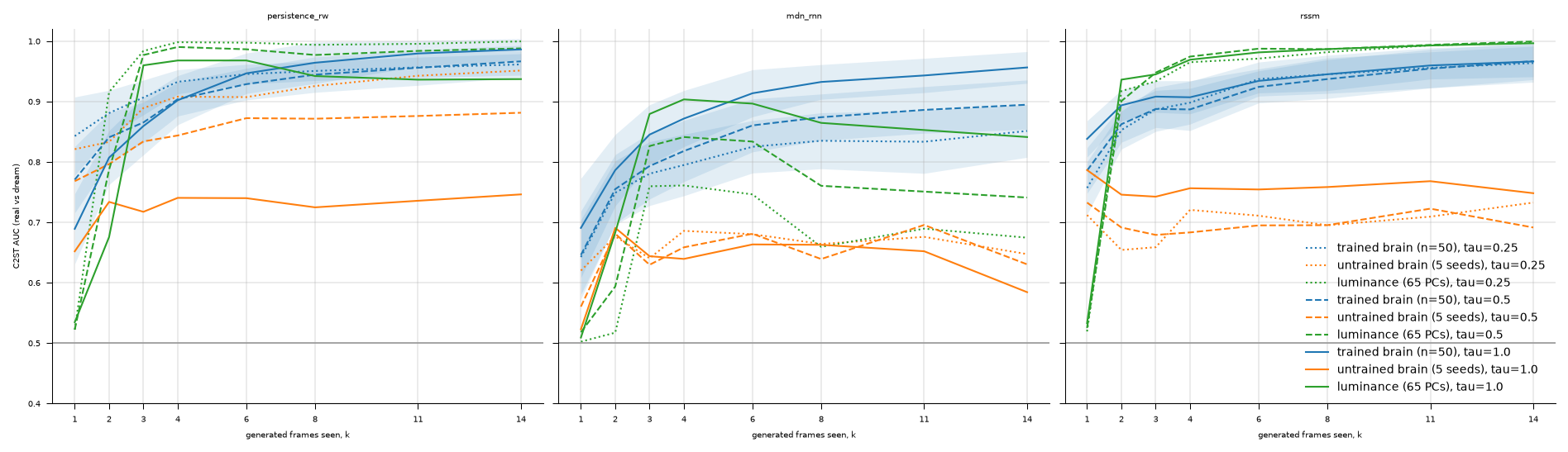
Caption: Detection horizon: two-sample-test AUC against the number $k$ of generated frames the features are computed over, one panel per world model. Blue: trained observer, mean over the 50 models with a $ 1$ standard deviation band; orange: the untrained observer, mean over the five seeds; green: the direct-luminance control. Line style encodes the temperature (dotted 0.25, dashed 0.5, solid 1.0). The grey line is chance. At $k = 1$ the features use only the mean and the mean step-to-step change (two integration steps); the luminance control at $k = 1$ uses the mean of a single frame.
Why It Matters: The horizon plot shows how quickly separability grows, distinguishing the slower MDN-RNN conditions from persistence and RSSM cases whose full-window AUCs are all high.
fig:probes
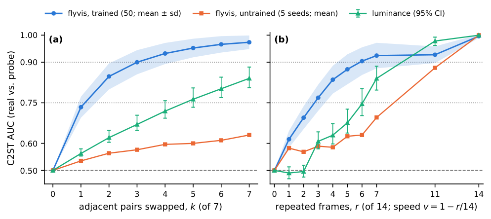
Caption: Graded temporal probes: two-sample-test AUC against the strength of the probe. (a) Number $k$ of the seven adjacent pairs of generated frames that are swapped; (b) number $r$ of the 14 generated frames that repeat their predecessor in slow motion (speed $v = 1 - r/14$; $r = 14$ is a freeze on the last context frame). Blue: trained observer, mean over the 50 models with a $ 1$ standard deviation band; orange: untrained observer, mean over the five seeds; green: direct-luminance control with its 95\% sequence-cluster bootstrap interval. Dotted lines mark the threshold levels 0.75 and 0.9, the dashed line chance. Strength zero is reality itself, where the AUC is 0.5 by construction.
Why It Matters: The probes isolate temporal-order defects using real frames, demonstrating that the trained response features can detect some small perturbations when the pixel-statistics control remains near chance.
🔮 Conclusion
In this setup, optic-flow training makes temporal differences in selected world-model rollouts more linearly decodable from the fly visual-system model’s response statistics. The trained responses distinguish all nine dreams, including on sequences not used to train the observer, and graded probes show sensitivity to small order changes.
The result is best read as an observer-referenced evaluation axis. The trained response representation and its detection horizon capture temporal deviations that pixel error does not order well. The study does not establish that the fly itself detects such continuations, that the connectome uniquely accounts for the signal, or that this measure predicts usefulness for control.
🛠️ Future Research Improvements
The paper points to testing other connectome-constrained brain models as validated models become available, asking whether a more complete brain carries more of the deviations and where in the model those signals occur. Such work would need comparable stimuli and carefully matched observer and classifier protocols to distinguish changes in the model from changes in the input distribution.
A second direction is a closed-loop experiment: use a fixed readout of motion-detector responses, such as a left-right difference in T4/T5 populations, to steer a generator’s viewpoint, then measure detection horizon as interaction proceeds. That would address a question absent from the current fixed-observer setup, but would still require a clear distinction between model behavior and animal behavior.
The authors also propose extending the benchmark to stronger world models. The current full-length AUC saturates for some generators, so the horizon curve may provide more range. Large pretrained video models require a matched null in which real frames pass through the same autoencoder, as the paper notes. Further work should broaden visual domains, lengthen rollouts, and test whether the reported response-space differences survive those changes.
🏭 Potential Industry Use Scenarios
A plausible engineering use is as an auxiliary temporal-fidelity probe for video world models. A team could freeze a task-trained visual encoder, generate continuations from held-out contexts, and train a simple two-sample classifier on response statistics to reveal temporal defects that pixel error or frame-change averages may rank differently. The paper’s detection-horizon setup could also help compare how quickly different generators diverge from real sequences, especially where full-window separability is already high.
The evidence supports only a research prototype in the paper’s narrow setting: MPI-Sintel luminance rendered to a flyvis retina, with three small generators and short continuations. Before using such a probe in production, builders would need to validate it on their target video domain, compare it with task-relevant and generic feature baselines, and check sensitivity to the chosen encoder and classifier. The paper does not demonstrate a deployed product, operational monitoring system, or improvement to downstream control, so these scenarios are prospective applications of its measurement design.
💬 Critical Analysis
The experimental design has useful controls: the same network before training, a direct-luminance feature control, sequence-disjoint validation, and graded probes made from real frames. The latter helps separate sensitivity to temporal order from gross visual differences in generated content. Reporting detection horizons also addresses saturation in full-window AUC and makes the generator comparison more informative.
The interpretation must remain narrow. The logistic regression, not the observer, makes the classification decision; the AUC indicates linear decodability in chosen response statistics. It is not a perceptual judgment, and the extracted cell-type weights are descriptive rather than mechanistic evidence. Moreover, the trained and untrained comparison does not isolate the connectome’s contribution, while the untrained seeds vary only in bias initialisation. The 50 trained models share data, wiring, and procedure, so they are an ensemble of related observers rather than independent replications.
The evaluation uses one visual dataset and short continuations, while the generators are small and the RSSM outputs decoder means. Stronger generators, other domains, longer horizons, autoencoder-matched controls, and comparisons with generic motion representations remain open. The authors also caution that some graded-probe thresholds interpolate across a coarse grid and need not be monotone. Finally, no code or result files are released with the preprint, which limits independent reproduction from the paper alone.