
📌 Highlights
CATF addresses context-aware forecasting, where one target series is predicted from its own history and aligned contextual variables. Its central design is a Transformer Manager that hard-routes each input to one specialized Worker.
The reported evaluation spans Weather, PM2.5-LA, PM2.5-RV, Bike Share, and Appliances, with horizons of 96, 192, 336, and 720 and both global and sample normalization. CATF improves over its standalone counterpart in 162 of 200 comparisons, and the best CATF-enhanced model wins 19 of 20 best-baseline comparisons.
The strongest interpretability evidence comes from Bike Share: day of week changes 37% of routing decisions when shuffled, compared with 10% for an untrained Manager, while the selected Worker is 9–23% more accurate than the alternatives on its routed samples.
The main caveats are increased training cost, dataset-dependent Worker count, and mostly non-significant ablation differences.
- Hard sample-level routing keeps inference to one Worker per forecast.
- Workers can reuse existing forecasters such as Informer, Autoformer, FEDformer, TimesNet, and iTransformer.
- The framework improves both accuracy and direct interpretability of model specialization.
- Time-MoE remains better in five of the 20 comparison settings, mostly at longer horizons.
🎯 Introduction
The paper defines context-aware time-series forecasting as predicting a single target variable from its history and contextual variables that affect its dynamics. Examples include bike demand driven by weather and calendar variables, air quality influenced by meteorology and co-pollutants, and appliance energy use affected by indoor and outdoor conditions. This differs from standard multivariate benchmarks in which variables of the same type are forecast jointly.
The authors argue that heterogeneous contexts create distinct temporal regimes that are difficult for a single model to capture. Ensemble methods require manual segmentation and aggregation, while Mixture-of-Experts systems require careful gating and can suffer from expert under-utilization. Large time-series foundation models provide general representations but may be expensive to adapt and brittle under distribution shifts.
CATF's objective is to learn model specialization directly from data. A Manager selects the most suitable Worker for each input, and Workers are trained on the samples assigned to them. The intended result is a combination of adaptive specialization, lower inference activation than a full ensemble, and routing decisions that can be inspected directly.
🔬 Methodology
For each forecast origin, the model receives a target-history window X and a context-history window C, both of length L. The target horizon Y contains the next Ly target values. The context variables are used only as inputs; CATF does not forecast their future values. Inputs are normalized either globally using training-split statistics or per sample using statistics from the input window, and predictions are inverse-transformed before evaluation.
The Manager is a K-class Transformer classifier. Feature encoding applies a linear projection, layer normalization, ReLU, and dropout. Transformer encoder layers model temporal-contextual dependencies, after which last-timestep pooling, a decoder, and softmax produce routing probabilities. The selected Worker is k*=arg max_i P_i and predicts the target sequence from the same X and C. The architecture is shown in the Manager-Worker diagram.
Training is deliberately ordered. Every Worker first produces a forecast and loss. These losses, together with each Worker's training volume, produce a soft routing target. The Manager is trained against that target, then routes each sample, and only the selected Worker is updated. The loss-based target and its volume-aware regularization are defined by Equations 2 and 3. The Manager uses Wasserstein distance, KL divergence, and parameter regularization, while Workers use forecasting MSE.
The procedure is modular: the main experiments use three identical Workers for each baseline architecture, while heterogeneous mixtures are also tested. The iterative procedure is summarized in Algorithm 1 and operationalized in the training-flow figure.
equation 2
Meaning: This constructs a loss-based pseudo-target for the Manager: Workers with lower losses receive larger routing probabilities.
equation 3
Meaning: This is the regularized pseudo-target used in the main training procedure. It combines Worker performance with an exploration term that favors underused Workers.
equation 5
Meaning: This Wasserstein distance measures the discrepancy between the Manager's predicted routing distribution and the pseudo-target with a geometry-aware objective.
equation 6
Meaning: The KL divergence penalizes mismatches where the Manager assigns low probability to Workers favored by the pseudo-target.
Iterative Training Process of CATF
Steps: ['Initialize the Manager and K Workers.', "For each mini-batch, compute every Worker's forecasting loss.", 'Construct the pseudo-target distribution P and update the Manager.', 'Use the updated Manager to select one Worker for each sample with arg max.', 'Partition the mini-batch by selected Worker and update only the corresponding Worker sub-batches.', 'Validate the models and save the best checkpoint when validation performance improves.']
Why It Matters: The procedure is the mechanism that turns loss-based competition into context-specific Worker specialization while retaining hard routing at inference.
📊 Experiments
The evaluation uses five context-rich datasets: Weather with CO2 as the target and 20 meteorological context variables; PM2.5-LA and PM2.5-RV with air-quality, meteorological, reanalysis, and co-pollutant context; Bike Share with calendar and weather context; and Appliances with room-level, lighting, and outdoor weather context. Samples are split chronologically into 80% training, 10% validation, and 10% testing. The look-back length is L=96 and horizons are Ly∈{96,192,336,720}.
Baselines are Informer, Autoformer, FEDformer, TimesNet, and iTransformer. CATF-enhanced variants use the same Worker configurations as their corresponding baselines, with three Workers in the main experiments. The comparison also includes the publicly released Time-MoE-50M checkpoint in a zero-shot setting. Each experiment is repeated over five independent runs, and the metric is original-scale MSE, where lower is better.
Across the 100 baseline-CATF pairs under global normalization, CATF wins 80; under sample normalization, it wins 82. At horizons 96, 192, 336, and 720, the global-normalization win counts are 23, 20, 19, and 18 out of 25, while the sample-normalization counts are 23, 20, 20, and 19. The best CATF-enhanced model wins 19 of 20 best-baseline settings and 15 of 20 Time-MoE settings.
The ablation on PM2.5-RV evaluates the Manager loss, regularization, Manager size, Worker count, and heterogeneous mixtures. The default MSE is 80.52 ± 1.02. KL-only and Wasserstein-only variants increase MSE by 1.7% and 1.3%, respectively; K=6 decreases MSE by 1.4%, while K=9 increases it by 2.6%. None of these differences is statistically significant in the reported test.
tab:best
Caption: Best standalone baseline vs. best CATF-enhanced model vs. zero-shot Time-MoE. For each setting, the best baseline and best CATF-enhanced model are selected over five model types and two normalization schemes; the better normalization scheme is used for Time-MoE.
| Dataset | Ly | Best baseline model | Best baseline MSE | Best CATF-enhanced model | Best CATF MSE | Time-MoE MSE |
|---|---|---|---|---|---|---|
| Weather | 96 | iTransformer | 204.7G | CATF-Informer | 155.7S | 164.9S |
| Weather | 192 | iTransformer | 249.3G | CATF-Informer | 220.8S | 215.0S |
| Weather | 336 | iTransformer | 254.6G | CATF-iTransformer | 232.3G | 225.6S |
| Weather | 720 | TimesNet | 269.1G | CATF-iTransformer | 235.9G | 233.5S |
| PM2.5-LA | 96 | iTransformer | 36.08S | CATF-iTransformer | 35.20S | 39.66S |
| PM2.5-LA | 192 | TimesNet | 40.16G | CATF-TimesNet | 39.25S | 43.16S |
| PM2.5-LA | 336 | TimesNet | 45.91G | CATF-TimesNet | 44.67S | 51.37G |
| PM2.5-LA | 720 | Informer | 52.81G | CATF-Informer | 51.37G | 60.59G |
| PM2.5-RV | 96 | iTransformer | 78.83S | CATF-TimesNet | 73.83S | 78.68G |
| PM2.5-RV | 192 | TimesNet | 87.78G | CATF-TimesNet | 83.44G | 87.28G |
| PM2.5-RV | 336 | TimesNet | 93.31G | CATF-TimesNet | 91.94G | 91.45G |
| PM2.5-RV | 720 | TimesNet | 85.81S | CATF-TimesNet | 86.12S | 87.41G |
| Bike Share | 96 | iTransformer | 15,134S | CATF-iTransformer | 14,258S | 15,802S |
| Bike Share | 192 | TimesNet | 20,500S | CATF-FEDformer | 19,930G | 20,044G |
| Bike Share | 336 | iTransformer | 27,477S | CATF-FEDformer | 23,498G | 23,512G |
| Bike Share | 720 | FEDformer | 34,864G | CATF-FEDformer | 32,858G | 30,793G |
| Appliances | 96 | iTransformer | 8,095G | CATF-Informer | 7,950G | 8,954G |
| Appliances | 192 | iTransformer | 8,123G | CATF-Informer | 7,739G | 8,596G |
| Appliances | 336 | iTransformer | 7,847G | CATF-Informer | 7,681G | 8,145G |
| Appliances | 720 | iTransformer | 8,046G | CATF-Informer | 7,870G | 8,511G |
| CATF Win | 20 settings | — | — | 19/20 vs. best baseline; 15/20 vs. Time-MoE | — | — |
| Impr. (%) | 20 settings | — | +5.9 | — | +4.9 vs. Time-MoE | — |
Why It Matters: This table contains the primary cross-dataset comparison and shows both the breadth of CATF's gains and the longer-horizon cases where Time-MoE remains stronger.
tab:ablation
Caption: Ablation study of CATF-iTransformer on PM2.5-RV (global normalization, L=Ly=96). MSE is mean ± SD over 5 runs without fixed random seeds; Δ is the relative change in mean MSE with respect to the default; p is from Welch’s t-test against the default.
| Setting | MSE | Δ (%) | p |
|---|---|---|---|
| Default | 80.52 ± 1.02 | — | — |
| KL only | 81.87 ± 2.75 | +1.7 | 0.347 |
| Wasserstein only | 81.56 ± 1.10 | +1.3 | 0.157 |
| No regularization | 80.94 ± 1.19 | +0.5 | 0.559 |
| Small Manager (d_model=128) | 81.23 ± 0.78 | +0.9 | 0.252 |
| Large Manager (d_model=768) | 81.05 ± 0.81 | +0.7 | 0.386 |
| K=6 | 79.37 ± 1.14 | −1.4 | 0.132 |
| K=9 | 82.61 ± 2.99 | +2.6 | 0.200 |
| Top-3 models (K=3) | 81.63 ± 2.13 | +1.4 | 0.334 |
| Top-2 models ×2 (K=4) | 80.04 ± 2.70 | −0.6 | 0.728 |
Why It Matters: The ablation tests whether the Manager objective, capacity, Worker count, and Worker heterogeneity materially affect performance.
equation 1
Meaning: This is the reported evaluation metric. Predictions are inverse-normalized before error is computed, so lower MSE indicates better accuracy in the target's original units.
align 7
Meaning: The Manager objective combines distribution matching through Wasserstein distance and KL divergence with a parameter regularization term.
fig:arch
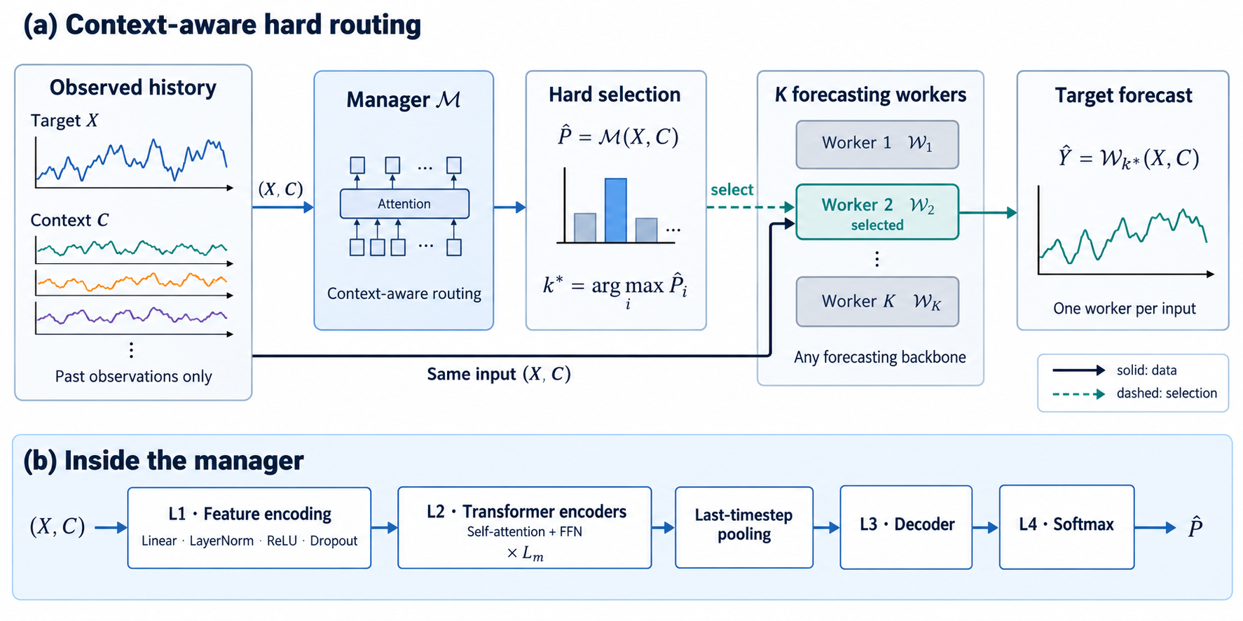
Caption: Manager–Worker architecture of CATF. (a) Given the target history X and the context history C, the manager M outputs routing probabilities P over the K workers. The worker with the highest probability, W_k*, receives the same input (X, C) and alone predicts the future target sequence Y. (b) Inside the manager: feature encoding (L1), L_m Transformer encoder layers (L2), last-timestep pooling, a decoder (L3), and softmax (L4).
Why It Matters: This figure defines the core execution path: the Manager sees the full input, selects one Worker, and avoids executing the other Workers at inference.
fig:training
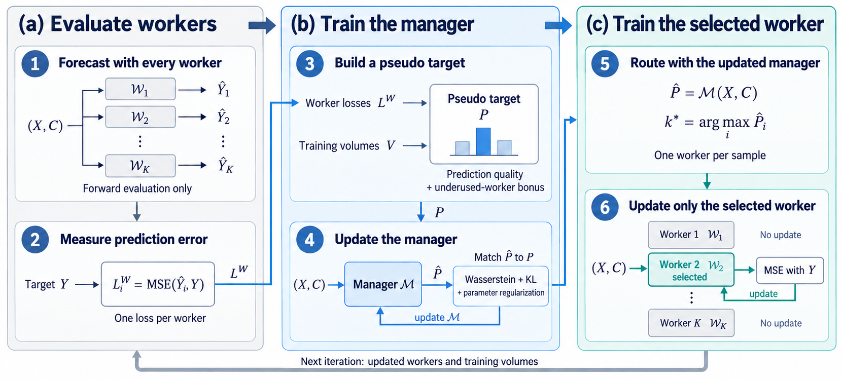
Caption: Iterative training of CATF, illustrated for one sample. (a) All workers first produce forecasts and losses (steps 1–2). (b) Their losses and training volumes define a pseudo target (step 3) that supervises the manager update (step 4). (c) The updated manager then selects one worker (step 5), and only that worker is trained on the sample (step 6).
Why It Matters: The training flow explains how CATF obtains routing supervision without manually labeled context regimes and how selective Worker updates create specialization.
app:bike_routing
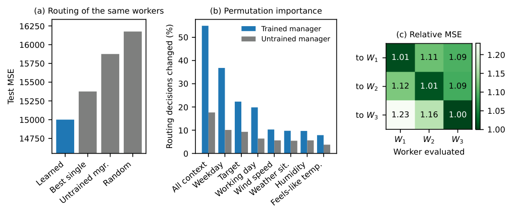
Caption: Routing of CATF-iTransformer on Bike Share (mean over 5 runs). (a) Test MSE of the same trained workers under the learned routing, the best single worker for all samples, an untrained manager, and random routing with the same worker shares. (b) Share of routing decisions that change when one variable is shuffled across test samples in the manager input only (top 8 of 12 inputs; “All context” shuffles all context variables at once), for the trained and an untrained manager. (c) MSE of each worker on the samples routed to each worker, divided by the lowest MSE in the row and averaged over runs.
Why It Matters: The figure tests whether routing itself improves forecasts, identifies which inputs drive routing, and checks whether each selected Worker is best on its assigned samples.
app:bike_profiles
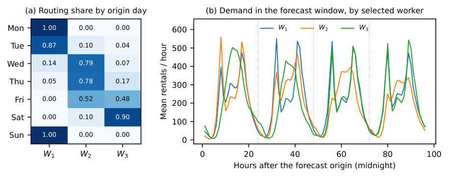
Caption: What each worker of CATF-iTransformer handles on Bike Share (one run). (a) Share of the forecasts made on each day of the week that are routed to each worker. (b) Mean bike rentals in the 96-hour forecast window for the forecasts made at midnight, grouped by the selected worker. W1 handles the forecasts made on Sunday to Tuesday, whose window consists mostly of working days (29 forecasts, on average 3.4 working days in the window); W2 handles the forecasts made on Wednesday to Friday, whose window reaches into the weekend (29 forecasts, 2.3 working days); W3 handles the forecasts made on Friday and Saturday, whose window starts with the weekend (11 forecasts, 1.9 working days).
Why It Matters: The Worker profiles provide a concrete qualitative interpretation of specialization: routing partitions the week according to the calendar composition of the forecast horizon.
🔮 Conclusion
CATF presents a practical way to add context-dependent specialization to existing time-series forecasters. Its Manager-Worker structure uses hard routing, trains Workers on routed subsets, and keeps only one Worker active for each inference example.
The reported results support the main claim: CATF improves its standalone counterpart in most dataset-horizon-normalization comparisons, the best CATF model wins nearly every best-baseline setting, and it exceeds zero-shot Time-MoE in most tested settings. The Bike Share analysis further suggests that routing decisions can correspond to meaningful calendar regimes rather than arbitrary partitioning.
The evidence is strongest for context-rich single-target forecasting with historical context available at inference. It does not yet establish universal gains, compute efficiency in wall-clock terms, or a reliable rule for selecting the number and composition of Workers.
🛠️ Future Research Improvements
A direct next step is adaptive Worker-count selection. The paper reports that K=6 slightly improves PM2.5-RV while K=9 degrades it, and suggests estimating the number of latent context regimes instead of fixing K globally.
Heterogeneous Workers need more targeted routing and regularization. Mixed architectures are not consistently beneficial and substantially degrade the Bike Share result in the reported analysis, so future work should identify when architectural diversity is complementary rather than disruptive.
Evaluation should expand to distribution shifts, missing or delayed context, longer horizons, more domains, and jointly forecasted multivariate settings. Compute-matched experiments should report training FLOPs, wall-clock time, memory, and inference latency alongside MSE.
The routing analysis could be strengthened with held-out regime labels, stability tests across random seeds, and explicit calibration or confidence measures for Manager decisions.
🏭 Potential Industry Use Scenarios
Air-quality monitoring is a direct use case: PM2.5 forecasting can route pollution windows to Workers specialized for different meteorological, reanalysis, and co-pollutant regimes. The PM2.5-LA and PM2.5-RV experiments provide the closest evidence for this scenario.
Shared-mobility operations can use calendar-aware routing for demand forecasting. The Bike Share case study indicates that Workers can specialize according to whether a forecast window contains mostly working days, a weekend transition, or a weekend start.
Building-energy management is another plausible deployment target. The Appliances dataset demonstrates a target driven by room-level conditions, lighting, and outdoor weather, where regime-specific forecasting could support scheduling or anomaly-aware planning.
Weather-station and industrial-monitoring systems may benefit when external variables change the target dynamics, but deployment should first verify that context history is available consistently and that the Manager's routing remains stable under operational shifts.
💬 Critical Analysis
The strongest aspect of CATF is the alignment between its mechanism and its interpretation claim. Because exactly one Worker produces each prediction, routing assignments are directly observable, and the Bike Share experiments compare learned routing against random routing, an untrained Manager, and a single Worker. The selected Worker is the most accurate on its assigned samples, with alternatives showing 9–23% higher MSE in the reported analysis.
The accuracy evidence is broad but should be interpreted with care. Results cover five datasets and four horizons, yet the best CATF variant changes by dataset and horizon. Time-MoE remains better in five settings, including several longer-horizon cases. The large Weather errors for some baselines are also affected by 50 missing-value codes in the training target, making raw cross-model comparisons on that dataset sensitive to training stability.
The ablations provide directional support for the combined Manager loss and default design, but all reported PM2.5-RV differences have p≥0.13. The experiment also uses five runs without fixed seeds, and heterogeneous mixtures can increase variance or degrade performance. These findings argue for cautious claims about which component is necessary.
Finally, CATF reduces inference activation to one Worker but increases training work by evaluating all Workers before selective updates and by using a larger epoch budget than the baselines. The paper does not quantify latency, memory, or energy, so the practical efficiency advantage remains a systems question rather than an established result.