
📌 Highlights
The paper studies whether pretrained Graph Foundation Models can be adapted for unsupervised multivariate time series anomaly detection (MTSAD). Its framework, GFM4MTSAD, keeps the graph backbone frozen and adds three coordinated components: SICA aligns temporal representations and graph structure, MAPS constructs screened pseudo-anomalies from local dependency breaks, and TGEC calibrates sensor and graph evidence against normal references before producing window scores. The method also outputs sensor-level localization evidence, addressing the need to identify which variables contribute to an alert.
The authors evaluate AnomalyGFM and OwlEye variants on MSL P-15, SMAP T-3, and SMD 1-1 against nine baselines, using AUROC, AUPRC, and F1 without point adjustment. Results vary by dataset and metric: OwlEye-based GFM4MTSAD reports 0.9246 AUROC, 0.6916 AUPRC, and 0.8138 F1 on MSL P-15; on SMAP T-3, PaAno reports a higher F1 than either proposed variant. The reported ablations support several design choices, while broader deployment behavior is not established.
- Three modules address input alignment, pseudo-anomaly supervision, and score calibration.
- The reported evaluation uses two GFM backbones and three benchmark entities.
- The paper reports strong results but not a uniform win across every metric.
🎯 Introduction
MTSAD is used to monitor systems where labeled failures are scarce and missed faults can have serious consequences. An anomaly may be a point deviation, a change in a sensor's temporal trajectory, or a breakdown in cross-sensor relationships. The paper therefore treats reliable window-level detection and sensor-level localization as related requirements. In the unsupervised setting studied here, training uses normal observations rather than labeled anomalies.
The authors describe two broad limitations in prior approaches. Temporal reconstruction or pattern-sensitivity methods can miss violations of inter-sensor structure, while graph-centric detectors model sensor relationships but commonly learn task-specific networks from limited target-domain data. Their learned graph can contain spurious edges, and transferring relational knowledge across systems is difficult. Pretrained GFMs such as AnomalyGFM and OwlEye offer reusable graph representations, but their graph inputs and token spaces do not directly match continuous, evolving time series.
The paper's objective is to adapt these pretrained models without discarding their relational priors or the time-series detail needed for detection. It identifies three linked obstacles: the feature and topology contract mismatch, unreliable supervision from generic pseudo-anomalies, and distortion when node responses are aggregated into window scores. GFM4MTSAD addresses those obstacles through SICA, MAPS, and TGEC, respectively. This is a paper-level adaptation proposal evaluated on three real-world dataset entities; claims about safety-critical deployment should be read as motivation rather than demonstrated operational outcomes.
🔬 Methodology
Given a window of sensor observations, a temporal frontend extracts per-sensor features and the Token Bridge projects them into the native input dimension of a frozen GFM. The projection is initialized from leading principal components of normal features. SICA then constructs a message-passing graph from absolute feature correlations regularized by edge frequencies measured on normal training graphs. Equation 1 defines this prior-weighted top-k graph. Because projection can discard temporal variation outside its subspace, IPRA computes the orthogonal residual and passes it through a gated low-rank correction, as specified in Equation 2. The backbone stays frozen while peripheral adapters and detection components are trained.
MAPS fits a sparse Graph-VAR model on normal data and generates localized interventions that alter lag behavior, neighbor contributions, relational orientation, or local evolution. It preserves the original prediction residual so that the synthetic window retains empirical background fluctuations. Equations 3 and 4 express the residual-preserving edit and its intervention primitives. Candidate windows are screened using standardized residual energy and edit magnitude; Equations 5 and 6 define the energy measure and constrained selection objective. The selected edited sensor set also supplies paired supervision for localization.
TGEC derives direct, local, relational, and context evidence, calibrates each against a normal reference distribution, and forms a multi-evidence consensus. Equation 7 maps a baseline score relative to normal references and applies the consensus only after the tail threshold is reached, preserving the baseline score for the rest of the distribution. Training includes contrastive learning, window ranking and classification, node ranking, and response-consistency terms; Equations 8 and 9 show the node-ranking term and combined objective. The framework outputs both a window score and auxiliary sensor evidence.
Equation 1: normal-prior graph construction
Meaning: Combines instantaneous feature correlations with normal-training edge frequencies, then applies the top-neighbor graph operator to form the message-passing topology.
Equation 2: IPRA residual recovery
Meaning: Defines the feature component outside the Token Bridge projection and adds a gated low-rank correction to the GFM node representations.
Equation 3: residual-preserving intervention
Meaning: Edits a sensor's predicted component within an intervention interval while retaining the empirical residual from the original series.
Equation 4: MAPS intervention primitives
Meaning: Specifies the lag, neighbor, relation, and local prediction changes used to synthesize candidate pseudo-anomalies.
📊 Experiments
The authors evaluate on Mars Science Laboratory telemetry entity MSL P-15, Soil Moisture Active Passive telemetry entity SMAP T-3, and Server Machine Dataset entity SMD 1-1. The reported dataset table lists 55, 25, and 38 variables, respectively, along with train/test counts and window/anomaly counts. Sequences are divided into their original train and test partitions, then segmented into windows of length 60 and stride 1. A test window is anomalous if it contains at least one anomalous timestamp. The anomaly-free training partition is further split: the first 80% is used for model fitting and reference construction, and the remaining 20% is held out for validation. Standardization uses training-block statistics.
The comparison includes nine baselines: SimCLR, CSI, SSD, AnomalyTransformer (AT), DCdetector, CTAD, CARLA, CAROTS, and PaAno. The proposed framework is instantiated with pretrained AnomalyGFM and OwlEye backbones. All methods use the same data partitions, labels, and evaluation protocol; timestamp-level baseline outputs are aggregated into window scores using within-window maximum. The reported metrics are AUROC, AUPRC, and F1 without point adjustment, with higher values indicating stronger discrimination and lower false-alarm overhead. The main comparison uses three runs per entity-backbone configuration. The reported training protocol includes a 30-epoch frontend warm start followed by 30 epochs of joint optimization.
In the main comparison, OwlEye-based GFM4MTSAD obtains the highest reported values among listed methods on MSL P-15: AUROC 0.9246, AUPRC 0.6916, and F1 0.8138. On SMAP T-3, the two proposed variants report AUROC 0.7233 and 0.7209, AUPRC 0.4120 and 0.4169, and F1 0.4922 and 0.4739; PaAno's reported F1 is 0.5505. On SMD 1-1, AnomalyGFM-based GFM4MTSAD has AUROC 0.9089, while OwlEye-based GFM4MTSAD has the higher AUPRC and F1, 0.6167 and 0.6198. Thus, the results are strong but depend on dataset, backbone, and metric.
Ablations with OwlEye report that removing PCA initialization or the IPRA residual bypass reduces AUPRC and F1 across the listed entities, while replacing boundary-ranked MAPS selection with random direct-edit selection lowers AUPRC on MSL and SMD. The normal graph prior is active only for the reported MSL ablation; the other two entries are dashes. TGEC comparisons across six configurations show that its effect is not uniformly beneficial on every metric/configuration: for example, MSL-O has 0.8366 AUPRC for both ECDF and TGEC, while global consensus is 0.1230. The authors also report that on SMD with OwlEye, at the normal-q99 threshold, TGEC reduces false positives from 918 to 599 (34.7%) while preserving true anomaly recall. These are dataset experiments, not evidence of live operational deployment.
tab:datasets
Caption: Statistics of the Evaluation Datasets.
| Dataset entity | Vars. | Train | Test | Windows | Anom. |
|---|---|---|---|---|---|
| MSL P-15 | 55 | 3,682 | 2,856 | 2,797 | 80 |
| SMAP T-3 | 25 | 2,876 | 8,579 | 8,520 | 302 |
| SMD 1-1 | 38 | 28,479 | 28,479 | 28,420 | 3,166 |
Why It Matters: It records the entity sizes and window/anomaly counts used in the evaluation.
tab:main-results
Caption: Performance Comparison of MTSAD on Three Benchmark Datasets. The Best and Second-Best Results are Highlighted in Bold and Underlined Text. AT Denotes AnomalyTransformer, G4M-A and G4M-O Denote Gfm4Mtsad Based on AnomalyGFM and OwlEye, Respectively.
| Dataset | Metric | SimCLR | CSI | SSD | AT | DCdetector | CTAD | CARLA | CAROTS | PaAno | G4M-A | G4M-O |
|---|---|---|---|---|---|---|---|---|---|---|---|---|
| MSL P-15 | AUROC | 0.5246 | 0.4659 | 0.4621 | 0.3072 | 0.3909 | 0.5420 | 0.6956 | 0.6592 | 0.5104 | 0.8747 | 0.9246 |
| MSL P-15 | AUPRC | 0.0280 | 0.0252 | 0.0255 | 0.0186 | 0.0215 | 0.0293 | 0.4208 | 0.0378 | 0.0271 | 0.1731 | 0.6916 |
| MSL P-15 | F1 | 0.0947 | 0.0805 | 0.0712 | 0.0569 | 0.0562 | 0.1029 | 0.5405 | 0.0950 | 0.0271 | 0.3318 | 0.8138 |
| SMAP T-3 | AUROC | 0.4956 | 0.5997 | 0.4543 | 0.5230 | 0.4717 | 0.5439 | 0.6654 | 0.4931 | 0.7923 | 0.7233 | 0.7209 |
| SMAP T-3 | AUPRC | 0.0650 | 0.0456 | 0.0691 | 0.2267 | 0.0382 | 0.0377 | 0.2841 | 0.0440 | 0.3908 | 0.4120 | 0.4169 |
| SMAP T-3 | F1 | 0.0814 | 0.0861 | 0.1189 | 0.3315 | 0.0799 | 0.0796 | 0.3897 | 0.0752 | 0.5505 | 0.4922 | 0.4739 |
| SMD 1-1 | AUROC | 0.5400 | 0.4114 | 0.6010 | 0.5423 | 0.5078 | 0.5451 | 0.3901 | 0.8740 | 0.5901 | 0.9089 | 0.8087 |
| SMD 1-1 | AUPRC | 0.1127 | 0.0932 | 0.2559 | 0.2632 | 0.1155 | 0.1200 | 0.2430 | 0.5225 | 0.1213 | 0.6050 | 0.6167 |
| SMD 1-1 | F1 | 0.2211 | 0.2006 | 0.3095 | 0.3530 | 0.2008 | 0.2126 | 0.2676 | 0.5625 | 0.2976 | 0.5680 | 0.6198 |
Why It Matters: The main comparison reports all three metrics for both backbones and nine baselines on each evaluated entity.
tab:ablation-joint
Caption: SICA and MAPS Ablations with the OwlEye Backbone (Native Window AUPRC and F1). Best and Second-Best Results Are Bold and Underlined, Respectively.
| Ablation variant | MSL-O AUPRC | MSL-O F1 | SMAP-O AUPRC | SMAP-O F1 | SMD-O AUPRC | SMD-O F1 |
|---|---|---|---|---|---|---|
| Full Model (SICA + MAPS) | 0.8131 | 0.9182 | 0.4519 | 0.5283 | 0.6932 | 0.6849 |
| w/ Minimal SICA + MAPS | 0.6998 | 0.8439 | 0.3408 | 0.4215 | 0.2483 | 0.3232 |
| w/o PCA Bridge Initialization | 0.4203 | 0.6854 | 0.3928 | 0.4784 | 0.6642 | 0.6344 |
| w/o Normal Graph Prior (λA = 0) | 0.6131 | 0.7526 | — | — | — | — |
| w/o IPRA Residual Bypass | 0.5723 | 0.8066 | 0.3410 | 0.4621 | 0.4756 | 0.5506 |
| w/ Random Direct-Edit Selection | 0.7555 | 0.8742 | 0.4277 | 0.5424 | 0.6445 | 0.6175 |
Why It Matters: The results quantify several SICA and MAPS ablations for the OwlEye backbone; dashes are preserved for inactive normal-prior cases.
fig:framework
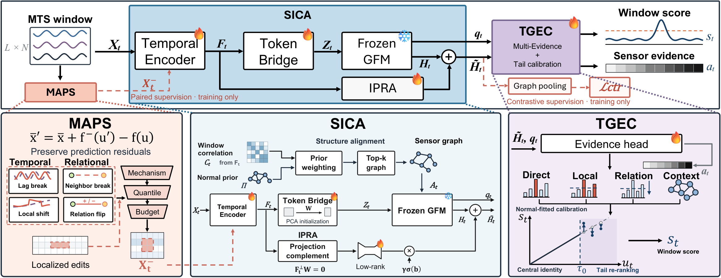
Caption: Overall architecture of Gfm4Mtsad. At a high level, Gfm4Mtsad adapts a frozen GFM to unsupervised MTSAD, outputting both window-level anomaly scores ($s_t$) and sensor-level localization evidence ($a_t$). Specifically, (1) MAPS (left, training only) synthesizes mechanism-aligned hard pseudo-anomalies ($X_t^-$) via residual-preserving interventions and multi-criteria screening to provide paired and contrastive supervision; (2) SICA (center) bridges the temporal-topological gap through prior-guided structure alignment, a Token Bridge, and orthogonal IPRA residual compensation while keeping the GFM backbone frozen; and (3) TGEC (right) integrates multi-granularity anomaly evidence via normal-c...
Why It Matters: The architecture figure shows how the training-only MAPS stage supplies pseudo-anomalies, SICA adapts inputs around a frozen backbone, and TGEC converts calibrated evidence into window and sensor outputs.
fig:intro
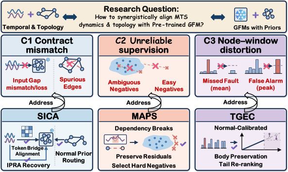
Caption: Left: Three key challenges in adapting pretrained GFMs to MTSAD and their solutions: (C1) Contract mismatch, addressed by SICA through representation alignment and normal prior routing; (C2) Unreliable supervision, addressed by MAPS through dependency disruption and hard-negative selection; and (C3) Node-window distortion, addressed by TGEC through normality-guided tail calibration. Right: AUROC comparison across three benchmarks against nine representative baselines, where G4M-A and G4M-O instantiate Gfm4Mtsad with pretrained AnomalyGFM and OwlEye backbones.
Why It Matters: It connects the three design challenges to the proposed modules and gives a visual overview of the reported AUROC comparisons.
fig:TGEC-mechanism
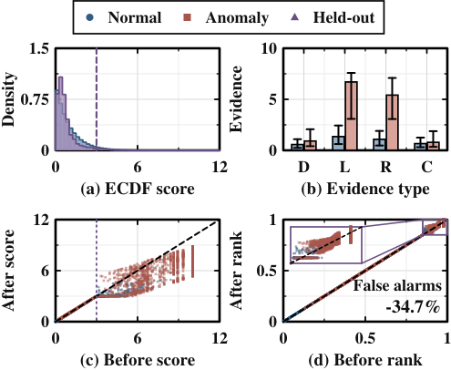
Caption: TGEC on SMD ( Gfm4Mtsad-O): (a) normal distributions and tail gate; (b) evidence medians and IQRs (D/L/R/C: direct/local/relation/context); (c) score mapping; (d) rank changes with the upper tail enlarged (both axes: 0.85--1). Normal/anomalous tail windows: 2,010/2,097. At the normal-q99 threshold, false positives decrease from 918 to 599 (34.7\%).
Why It Matters: The figure illustrates the authors' SMD analysis of tail-only calibration and reports a decrease in false positives at the stated normal-q99 threshold.
fig:TGEC-scoring-ablation
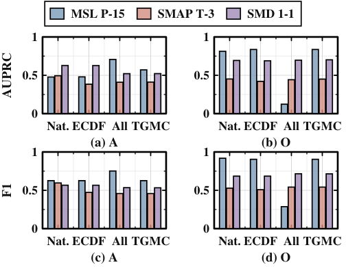
Caption: TGEC scoring ablation: top, AUPRC; bottom, raw oracle F1. A/O denote Gfm4Mtsad-A/O. Nat.: native scores; ECDF: normal-reference scoring; All: global consensus; TGEC: tail consensus.
Why It Matters: It compares native, ECDF, global-consensus, and TGEC scoring variants, visualizing the trade-off behind restricting evidence fusion to the tail.
fig:TGEC-tail-mass
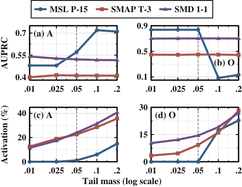
Caption: Tail-mass sensitivity: top, AUPRC; bottom, test-window tail activation. A/O denote Gfm4Mtsad-A/O. The fusion weight is fixed at 0.5. Dashed lines mark the default tail mass of 0.05. Horizontal axes are logarithmic; vertical ranges vary by panel.
Why It Matters: This sensitivity figure relates the selected normal-reference tail mass to AUPRC and test-window activation.
fig:ipra-rank
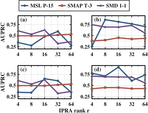
Caption: IPRA rank sensitivity: native AUPRC at validation-selected (top) and final (bottom, epoch 30) checkpoints. Left/right: Gfm4Mtsad-A/O. Dashed lines mark the default rank of 16. All panels share the vertical scale; ranks are spaced logarithmically.
Why It Matters: The authors use this figure to examine how the capacity of IPRA's residual pathway affects native AUPRC across both backbones.
🔮 Conclusion
The paper presents GFM4MTSAD as a way to adapt frozen pretrained graph models to unsupervised MTSAD. Its SICA module aligns time-series features and topology while recovering projection-excluded information; MAPS supplies screened, residual-preserving pseudo-anomalies; and TGEC calibrates multi-granular evidence while preserving the central score distribution. Experiments with AnomalyGFM and OwlEye across MSL P-15, SMAP T-3, and SMD 1-1 show strong results relative to the included baselines, with performance varying by dataset and metric. The authors conclude that coordinated temporal and relational adaptation can make pretrained graph models effective anomaly-detection backbones.
🛠️ Future Research Improvements
The authors identify three future directions. First, they plan to study how native token capacity and pretraining inductive biases affect transfer across heterogeneous GFMs, which could motivate adaptation strategies that coordinate representation granularity with backbone capacity. Second, they propose unified pretraining across time series and graphs so continuous temporal dynamics and discrete topology can be learned in a shared latent space rather than bridged only at downstream adaptation time. Third, they point to continual adaptation under non-stationary regimes and distribution shifts, with graph priors and tail-calibration references evolving online while retaining pretrained knowledge.
These directions also suggest concrete evaluations before a production setting can be assessed: measure performance across more entities and operational regimes; test whether the learned normal graph prior remains useful after sensor relationships change; and quantify how often reference updates alter alerts under benign drift. The paper does not report these evaluations, so they should be treated as open research questions rather than demonstrated capabilities. A useful extension would also report localization quality against sensor-level fault labels, since the supplied benchmark results emphasize window-level metrics.
🏭 Potential Industry Use Scenarios
The paper motivates MTSAD in mission-critical industrial control, healthcare, and finance, where anomalies may be sparse and labels expensive. Its experiments specifically cover spacecraft telemetry from MSL P-15 and SMAP T-3 and industrial server monitoring from SMD 1-1. Within those settings, a window-level alert paired with sensor-level evidence could help an operator prioritize a fault and inspect variables associated with the event. The authors' SMD mechanism analysis also examines reducing false positives at a fixed normal-reference threshold, a practical concern for alert queues.
These results support evaluating the method as an offline monitoring component or as a decision-support prototype in telemetry and server operations. They do not establish performance in deployed control loops, healthcare systems, or financial monitoring, and no live operational study is reported. A team considering adoption would need to validate its anomaly definitions, threshold policy, sensor localization quality, runtime cost, and reference-update process on its own data. In particular, a frozen graph backbone does not by itself show that the full pipeline will tolerate changing equipment, sensor failures, or distribution shift.
💬 Critical Analysis
A strength of the work is that it treats input alignment, training supervision, and inference-time aggregation as connected parts of one adaptation problem. The modules have explicit roles, and the experiments include comparisons across two different pretrained backbones, three dataset entities, component ablations, TGEC scoring variants, and parameter sensitivity. The reported results are not presented as uniformly best: the proposed models differ in their relative strengths, and PaAno has the higher listed F1 on SMAP T-3. That variation is useful evidence that backbone and metric choice matter.
The ablations provide partial support for SICA and MAPS: removing PCA initialization or IPRA generally lowers the reported OwlEye metrics, and random direct-edit selection reduces AUPRC on MSL and SMD. The TGEC table is more mixed. On MSL-O, TGEC matches ECDF at 0.8366 AUPRC with zero reported tail activation, while global consensus falls to 0.1230; on other configurations, TGEC does not exceed every listed alternative. This suggests its value depends on the distribution of test scores and on which metric is examined, rather than guaranteeing a general improvement.
The evaluation is limited to three dataset entities and a three-run main comparison. The supplied results do not establish performance across all entities in the underlying datasets, other sensor domains, or non-stationary live operation. Some ablation cells are unavailable because the normal graph prior was inactive, limiting component attribution. The reported benchmark protocol also uses window labels and within-window maximum aggregation for baseline outputs; conclusions should be interpreted within that evaluation setup. Finally, the paper reports window-level detection metrics but the supplied main comparison does not provide a standalone quantitative sensor-localization metric. Reproduction and deployment studies should examine calibration stability, localization accuracy, computational overhead, and robustness when the normal reference no longer matches current operations.