
📌 Highlights
FARR treats the difference between a standard conditioned forecast and a matched null-condition forecast as evidence about how conditioning affects the prediction. A lightweight residual module then uses this evidence and recent history to make bounded, horizon-specific corrections.
- Best dataset-average MSE and MAE among the listed methods on ETTh1, Weather, Traffic, and ECL.
- Uses a frozen Qwen2.5-0.5B-Instruct-based forecaster and adds a small trainable refinement module.
- Dual endpoints improve over single-endpoint and disagreement-only ablations across the reported datasets.
- The main deployment cost is a second backbone pass, not the residual correction itself.
- Reported metrics are standardized-space MSE and MAE, and individual-horizon rankings are not uniformly dominated by FARR.
🎯 Introduction
Language-model-based forecasting uses auxiliary conditioning to incorporate additional information into numerical prediction, but the benefit of conditioning depends on the dataset and forecasting setting. Prior systems can produce a stronger representation or richer prompt while still making a particular forecast worse, and a standard pipeline exposes only the conditioned output rather than the change caused by conditioning.
FARR's paper-level objective is to make that change observable and useful for correction. It compares a valid forecast with a null-condition forecast, combines their disagreement with historical context, and learns when the disagreement should alter the final prediction. The objective is residual refinement around a valid forecast, not replacement of the frozen forecaster.
🔬 Methodology
For each forecast origin, the Endpoint Proposal Module runs the same frozen forecaster twice: once with standard conditioning and once with a fixed null operation. The two passes share the checkpoint, historical input, preprocessing, output settings, and sample order, so their difference isolates the conditioning intervention. The method then forms an 18-dimensional feature vector per horizon and channel from 168 recent observations, endpoint values, disagreement statistics, and normalized horizon position.
The shared residual refiner is a two-hidden-layer MLP with architecture \(18\rightarrow128\rightarrow128\rightarrow1\), GELU hidden activations, zero-initialized output, and tanh-bounded residuals. The disagreement features include signed and absolute differences, scale-normalized displacement, first-order change, smoothness, relative displacement, and sign consistency. Stage 2 can adjust the valid endpoint using bounded horizon parameters before recomputing endpoint-dependent features.
The Conservative Residual Composer uses a learnable horizon-specific gate capped at 0.20, so the residual correction remains bounded in standardized space. Training combines a final-forecast SmoothL1 term, a residual-target SmoothL1 term, residual smoothness, and residual L2 regularization. Stage 2 is retained only when validation MSE and MAE both improve over the valid forecast; otherwise the Stage 1 or valid forecast is retained.
tab:settings
Caption: Model hyperparameters and training settings.
| Setting | Value |
|---|---|
| Input / label / token length | 672 / 576 / 96 |
| Prediction horizon H | 96, 192, 336, 720 |
| History / recurrence window | 168 / 24 |
| Refiner architecture | 18 → 128 → 128 → 1 |
| Residual output | tanh; [−1, 1] |
| Gate cap / initial logit | 0.20 / −6 |
| SmoothL1 transition / αr | 1.0 / 0.10 |
| Smoothness / residual L2 weights | 0.01 / 0.01 |
| Adjustment scale / offset bounds | 0.10 / 0.10 |
| Batch size (train and evaluation) | 8192 |
| Weight decay / gradient clipping | 10−4 / 1.0 |
| Stage 1/2 learning rates | 10−3 / 10−4 |
| Stage 1/2 epochs; patience | 10/5; 2/2 |
Why It Matters: The settings table gives the concrete dimensions, bounds, optimization rates, and training budget for implementation.
equation 1
Meaning: Defines the matched valid and null endpoints.
equation 2
Meaning: Defines endpoint disagreement.
equation 5
Meaning: Defines the shared residual refiner and its bounded output.
equation 6
Meaning: Defines the bounded Stage 2 forecast adjustment.
📊 Experiments
The evaluation uses ETTh1, Weather, Traffic, and Electricity (ECL) with input length \(L=672\) and horizons \(H\in\{96,192,336,720\}\). A StandardScaler is fitted on the training split and applied unchanged to validation and test data. Locally evaluated MSE and MAE are computed in standardized space, and dataset averages weight the four horizons equally. Endpoint forecasts use a frozen Qwen2.5-0.5B-Instruct checkpoint with label length 576 and token length 96. Baselines include SE-LLM, TimeMixer++, Time-MoE, TQNet, TimeCMA, LLM-TS, AutoTimes, and Time-LLM.
FARR reports dataset-average MSE/MAE of 0.3773/0.4120 on ETTh1, 0.2208/0.2578 on Weather, 0.3790/0.2578 on Traffic, and 0.1520/0.2465 on ECL, the lowest dataset-average pair among the listed methods on all four datasets. Individual-horizon rankings vary: Time-MoE is lower on ETTh1 at horizon 96, SE-LLM is lower on ETTh1 at horizon 192, and Time-LLM has lower ECL MSE at horizon 720.
Ablations support the use of matched dual endpoints and the combined feature set. Dual-endpoint Stage 1 improves both metrics over the single-endpoint and disagreement-only variants on every dataset. Full FARR outperforms the parameter-matched MLP in all eight dataset–metric comparisons. Stage 2 improves six of eight comparisons over Stage 1, while ETTh1 MSE increases by 0.0003 and Weather MAE by 0.0001; the extra adjustment benefit therefore varies by dataset.
Sensitivity experiments vary \(\lambda_{\max}\), \(\alpha_r\), and the two regularizer weights while fixing architecture, seed, optimizer, and training budget. The paper reports larger MSE changes when residual refinement is disabled or regularization is increased. On ETTh1, the single-backbone configuration takes 63.03 ms, the extra endpoint adds 21.01 ms, the correction adds 1.08 ms, and full FARR takes 85.12 ms; the standardized MSE reduction relative to the local valid anchor is 0.0127.
tab:main
Caption: Long-horizon forecasting results (MSE/MAE). Red/blue mark the lowest/second-lowest values. Avg. averages the four displayed horizons; – denotes unreported results. ∗ denotes our reproduced results.
| Dataset | H | FARR (Ours) | SE-LLM | TimeMixer++ | Time-MoE | TQNet | TimeCMA | LLM-TS | AutoTimes | Time-LLM |
|---|---|---|---|---|---|---|---|---|---|---|
| ETTh1 | 96 | 0.353/0.393 | 0.352/0.393 | 0.361/0.403 | 0.349/0.379 | 0.371/0.393 | 0.373/0.391 | 0.403/0.420 | 0.360/0.397 | 0.362/0.392 |
| ETTh1 | 192 | 0.379/0.413 | 0.378/0.411 | 0.416/0.441 | 0.395/0.413 | 0.428/0.426 | 0.427/0.421 | 0.440/0.441 | 0.391/0.419 | 0.398/0.418 |
| ETTh1 | 336 | 0.385/0.413 | 0.391/0.420 | 0.430/0.434 | 0.447/0.453 | 0.476/0.446 | 0.458/0.448 | 0.471/0.457 | 0.408/0.432 | 0.430/0.427 |
| ETTh1 | 720 | 0.392/0.429 | 0.402/0.437 | 0.467/0.451 | 0.457/0.462 | 0.487/0.470 | 0.449/0.460 | 0.503/0.487 | 0.429/0.452 | 0.442/0.457 |
| ETTh1 | Avg. | 0.377/0.412 | 0.381/0.415 | 0.419/0.432 | 0.412/0.427 | 0.441/0.434 | 0.427/0.430 | 0.454/0.451 | 0.397/0.425 | 0.408/0.424 |
| Weather | 96 | 0.141/0.190 | 0.150/0.200 | 0.155/0.205 | 0.157/0.211 | 0.157/0.200 | 0.167/0.211 | 0.166/0.217 | 0.158/0.208 | 0.147/0.201 |
| Weather | 192 | 0.185/0.234 | 0.194/0.243 | 0.201/0.245 | 0.208/0.256 | 0.206/0.245 | 0.212/0.253 | 0.229/0.269 | 0.207/0.254 | 0.189/0.234 |
| Weather | 336 | 0.242/0.277 | 0.247/0.285 | 0.248/0.285∗ | 0.255/0.290 | 0.262/0.287 | 0.270/0.292 | 0.278/0.302 | 0.262/0.298 | 0.262/0.279 |
| Weather | 720 | 0.315/0.330 | 0.323/0.339 | 0.316/0.332∗ | 0.405/0.397 | 0.344/0.342 | 0.350/0.348 | 0.354/0.351 | 0.342/0.353 | 0.318/0.338∗ |
| Weather | Avg. | 0.221/0.258 | 0.229/0.267 | 0.230/0.267∗ | 0.256/0.289 | 0.242/0.269 | 0.250/0.276 | 0.257/0.285 | 0.242/0.278 | 0.229/0.263∗ |
| Traffic | 96 | 0.344/0.240 | 0.350/0.243 | 0.392/0.253 | – | 0.413/0.261 | – | 0.587/0.315 | 0.369/0.257 | 0.362/0.248 |
| Traffic | 192 | 0.367/0.252 | 0.373/0.254 | 0.402/0.258 | – | 0.432/0.271 | – | 0.612/0.326 | 0.394/0.268 | 0.390/0.288∗ |
| Traffic | 336 | 0.385/0.260 | 0.390/0.263 | 0.428/0.263 | – | 0.450/0.277 | – | 0.634/0.338 | 0.413/0.278 | 0.407/0.299∗ |
| Traffic | 720 | 0.420/0.279 | 0.429/0.285 | 0.441/0.282 | – | 0.486/0.295 | – | 0.640/0.351 | 0.449/0.299 | 0.430/0.288 |
| Traffic | Avg. | 0.379/0.258 | 0.386/0.261 | 0.416/0.264 | – | 0.445/0.276 | – | 0.618/0.333 | 0.406/0.276 | 0.397/0.281∗ |
| ECL | 96 | 0.124/0.218 | 0.130/0.225 | 0.135/0.222 | – | 0.134/0.229 | 0.143/0.238 | 0.167/0.271 | 0.140/0.236 | 0.131/0.224 |
| ECL | 192 | 0.136/0.233 | 0.148/0.242 | 0.147/0.235 | – | 0.154/0.247 | 0.161/0.259 | 0.178/0.280 | 0.159/0.253 | 0.152/0.241 |
| ECL | 336 | 0.155/0.251 | 0.164/0.259 | 0.164/0.245 | – | 0.169/0.264 | 0.169/0.261 | 0.198/0.302 | 0.177/0.270 | 0.160/0.248 |
| ECL | 720 | 0.193/0.284 | 0.203/0.293 | 0.212/0.310 | – | 0.201/0.294 | 0.219/0.315 | 0.233/0.344 | 0.216/0.303 | 0.192/0.298 |
| ECL | Avg. | 0.152/0.247 | 0.161/0.255 | 0.165/0.253 | – | 0.165/0.259 | 0.173/0.268 | 0.194/0.299 | 0.173/0.266 | 0.159/0.253 |
Why It Matters: The main table reports the complete horizon-level and dataset-average comparison.
tab:ablation
Caption: Component ablations in standardized space, averaged over four horizons. Best values are bold.
| Variant | ETTh1 MSE | ETTh1 MAE | Weather MSE | Weather MAE | Traffic MSE | Traffic MAE | ECL MSE | ECL MAE |
|---|---|---|---|---|---|---|---|---|
| Local valid anchor | 0.3900 | 0.4200 | 0.2300 | 0.2651 | 0.3865 | 0.2627 | 0.1605 | 0.2545 |
| Adjustment only | 0.3810 | 0.4151 | 0.2280 | 0.2661 | 0.3848 | 0.2609 | 0.1609 | 0.2540 |
| Matched MLP | 0.3796 | 0.4142 | 0.2258 | 0.2622 | 0.3835 | 0.2600 | 0.1584 | 0.2518 |
| History only | 0.3834 | 0.4170 | 0.2286 | 0.2668 | 0.3881 | 0.2635 | 0.1615 | 0.2549 |
| Single endpoint | 0.3818 | 0.4158 | 0.2270 | 0.2645 | 0.3856 | 0.2614 | 0.1602 | 0.2533 |
| Disagreement only | 0.3828 | 0.4164 | 0.2284 | 0.2659 | 0.3841 | 0.2607 | 0.1611 | 0.2545 |
| Dual endpoint (Stage 1) | 0.3770 | 0.4123 | 0.2230 | 0.2577 | 0.3821 | 0.2590 | 0.1562 | 0.2497 |
| Full FARR | 0.3773 | 0.4120 | 0.2208 | 0.2578 | 0.3790 | 0.2578 | 0.1520 | 0.2465 |
Why It Matters: The ablation table tests whether gains come from dual endpoints and the complete refinement design rather than from an extra MLP alone.
tab:latency
Caption: ETTh1 mean inference latency (ms) and standardized MSE reduction relative to the local valid anchor. Latency increments are differences between execution-mode means.
| Dataset | Single backbone | Extra endpoint | Extra correction | Full FARR | MSE reduction |
|---|---|---|---|---|---|
| ETTh1 | 63.03 | 21.01 | 1.08 | 85.12 | 0.0127 |
Why It Matters: The latency breakdown makes the deployment cost explicit.
fig:motivation
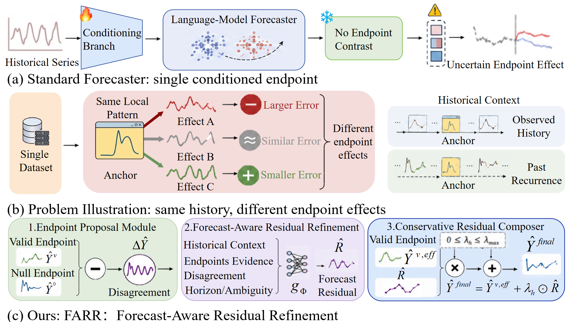
Caption: Motivation of FARR. (a) A single conditioned forecast does not reveal the prediction change relative to a null condition. (b) Conditioning can have different effects on forecasting error. (c) FARR combines endpoint evidence with historical features for residual refinement and applies horizon-wise gating before adding the residual to the effective valid forecast.
Why It Matters: This figure motivates why a matched null forecast is needed and shows how the observed conditioning effect becomes an input to residual refinement.
fig:framework
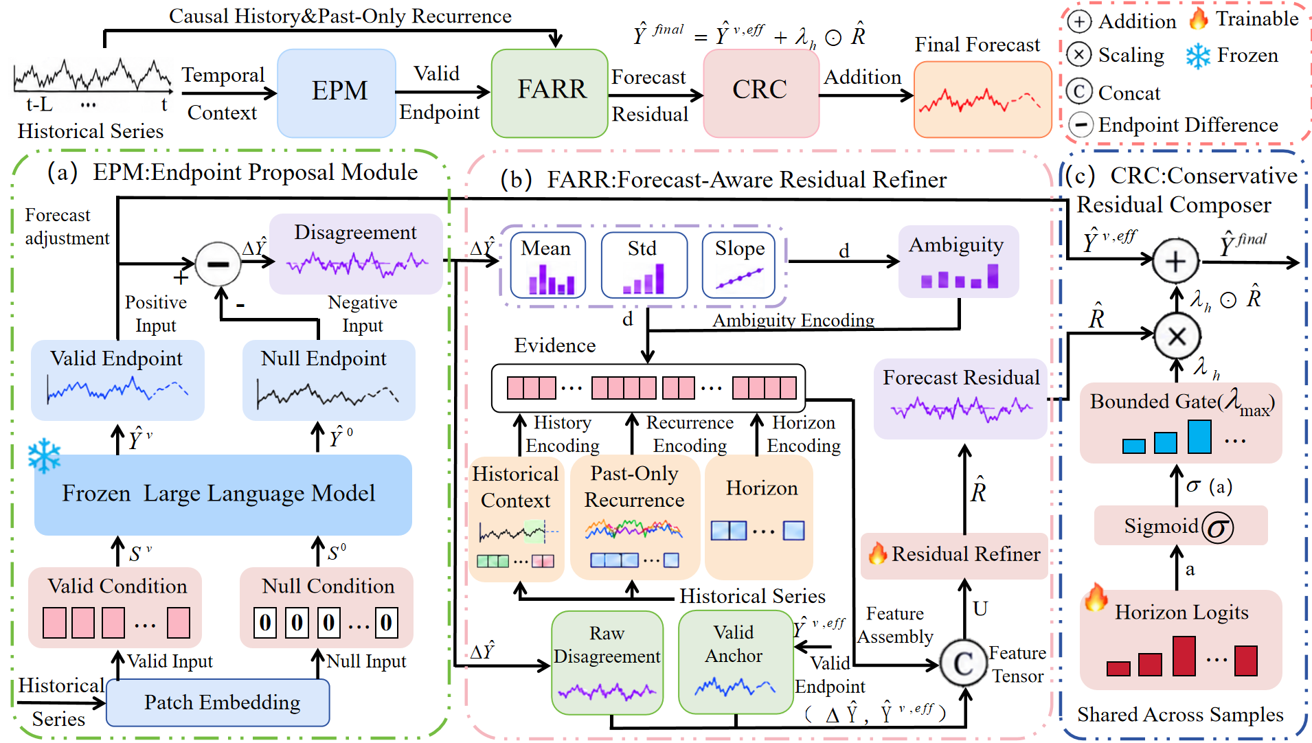
Caption: FARR architecture. EPM obtains matched endpoints, and forecast adjustment yields the effective valid forecast. The residual refiner combines endpoint evidence with historical context in $U$. CRC applies horizon-wise gating and adds the predicted residual to $ Y^v,eff$.
Why It Matters: The architecture view connects endpoint generation, residual prediction, forecast adjustment, and conservative gated composition.
fig:sensitivity
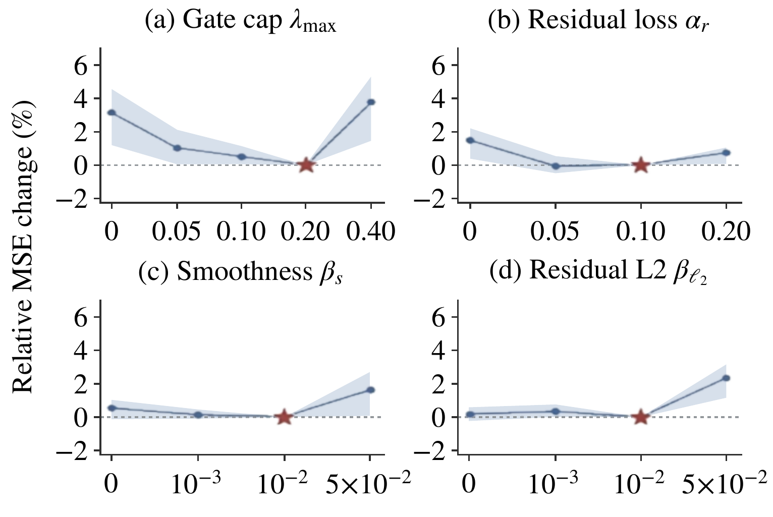
Caption: Hyperparameter sensitivity. Lines and shading show mean relative MSE changes and the 25th--75th percentile range across included forecasting settings. Stars mark the normalization reference.
Why It Matters: The sensitivity analysis indicates which refinement and regularization choices most affect standardized MSE across the evaluated settings.
🔮 Conclusion
FARR addresses the variable effects of auxiliary conditioning by learning residual corrections from matched valid and null forecasts plus historical context. Its shared refiner and bounded horizon-wise gates improve dataset-average performance while keeping the main forecasting backbone frozen.
Across four benchmarks, the paper reports the lowest dataset-average MSE and MAE among the compared methods. The principal trade-off is inference overhead from generating the additional endpoint, which motivates the paper's proposed follow-up directions.
🛠️ Future Research Improvements
The paper explicitly identifies selective endpoint generation and distillation as future directions for retaining endpoint-evidence benefits with lower inference cost. A natural implementation path is to learn when the null endpoint is likely to be useful and skip it for low-value cases, or to distill the two-endpoint correction into a single-pass model.
Further evaluation should test whether the mechanism transfers across frozen forecasters, conditioning pathways, seeds, and original-unit metrics. The current evidence supports the method on four standardized benchmark settings, but does not establish robustness under distribution shift or production latency constraints.
🏭 Potential Industry Use Scenarios
FARR could be integrated into long-horizon forecasting services that already expose an auxiliary-conditioning pathway, such as energy-load, electricity-demand, weather, or traffic forecasting systems. The architecture is attractive when the backbone must remain frozen and the organization can afford a second forecast pass for improved accuracy.
The benchmark results provide technical evidence for these domains but not deployment validation. Before production use, engineers should measure end-to-end latency, memory, cost per forecast, failure behavior when the valid and null endpoints disagree sharply, and performance in the original business units.
💬 Critical Analysis
The strongest aspect of FARR is its causal-style intervention within the forecasting pipeline: the null endpoint provides a concrete reference for measuring the conditioning-induced change, while history determines whether that change should be trusted. The ablations support the combined design, especially the improvement of dual-endpoint refinement over single-endpoint and disagreement-only variants.
The empirical case is promising but should be interpreted carefully. The main averages are in standardized space, some baseline entries are reproduced, and some table cells are unreported. FARR also leads on dataset averages even though other methods win selected individual horizons, so the aggregate advantage does not imply universal horizon-level dominance.
Reproducibility would benefit from broader backbone and seed coverage, confidence intervals, original-unit reporting, and controlled comparisons with identical evaluation pipelines. The paper states that code will be released, which should make it possible to verify the endpoint intervention, feature construction, stage-selection rule, and latency measurements.